Note
Click here to download the full example code
PyMAPDL Tutorial#
In this tutorial, we will introduce some of the capabilities of PyMAPDL applied to Aerospace students and advocates.
Python + Ansys = PyAnsys#
PyAnsys is Ansys effort on making their products accessible using Python programming language.
Today we will focus on PyMAPDL with is the Python library which exposes MAPDL (Ansys Structural).

What is PyMAPDL?#
PyMAPDL is the pythonic interface for Ansys MAPDL product.
What does this mean?
It means that you can call Ansys MAPDL functionalities (Solvers, Post processing tools, etc) using Python programming language.
MAPDL provides many tools and features which would require A LOT of time to explain, so let’s have a quick overview.
Launching PyMAPDL#
But first, let’s launch PyMAPDL.
from ansys.mapdl.core import launch_mapdl

mapdl = launch_mapdl()

print(mapdl)
Product:             Ansys Mechanical Enterprise
MAPDL Version:       22.2
ansys.mapdl Version: 0.63.2
Geometry#
PyMAPDL support points (keypoints), lines, areas, and volumes for geometry definition.
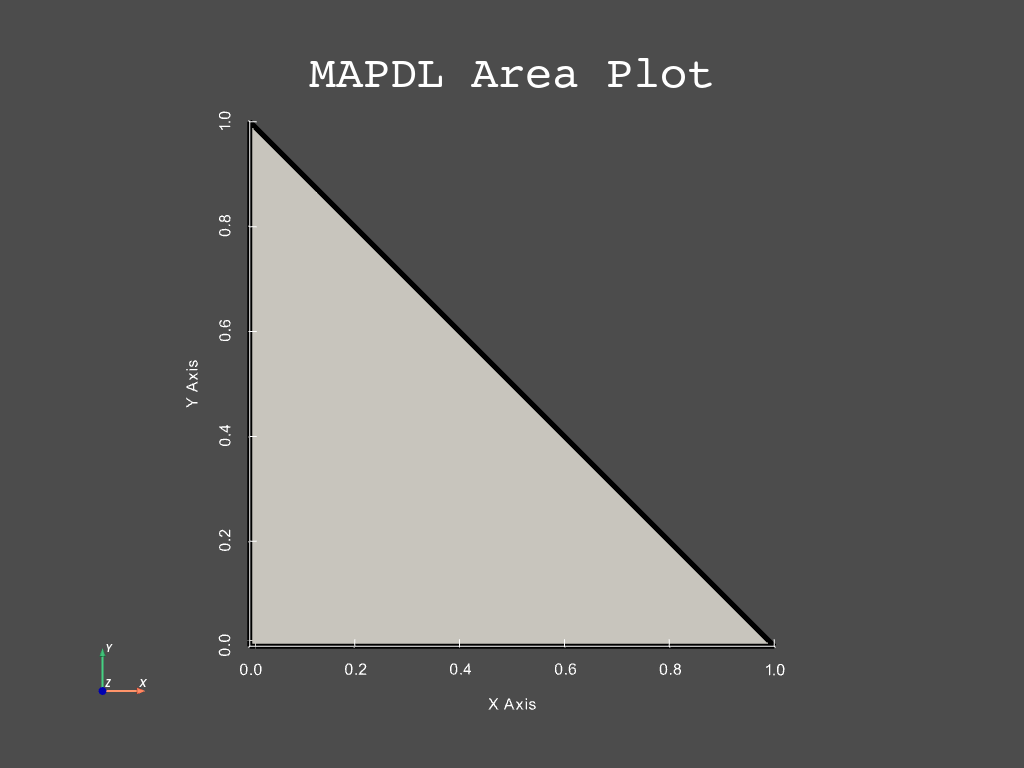
You can plot an area using keypoints:
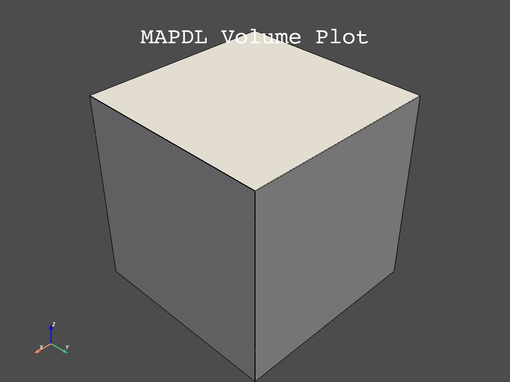
Create a simple cube volume.
mapdl.clear()  # let's clear first.
mapdl.prep7()  # entering in preprocessor

k0 = mapdl.k("", 0, 0, 0)  # defining a keypoint at (0,0,0) location
k1 = mapdl.k("", 1, 0, 0)  # defining a keypoint at (1,0,0) location
k2 = mapdl.k("", 1, 1, 0)  # etc
k3 = mapdl.k("", 0, 1, 0)
k4 = mapdl.k("", 0, 0, 1)
k5 = mapdl.k("", 1, 0, 1)
k6 = mapdl.k("", 1, 1, 1)
k7 = mapdl.k("", 0, 1, 1)

# defining volume according the kps
v0 = mapdl.v(k0, k1, k2, k3, k4, k5, k6, k7)

mapdl.vplot(show_lines=True)
Material definition#
You can define materials using the following commands:
# Define a material (nominal steel in SI)
mapdl.mp("EX", 1, 210e9)  # Elastic moduli in Pa (kg/(m*s**2))
mapdl.mp("DENS", 1, 7800)  # Density in kg/m3
mapdl.mp("NUXY", 1, 0.3)  # Poisson's Ratio
MATERIAL 1 NUXY = 0.3000000
At any point you can use help to get information about each function
help(mapdl.mp)
Help on method mp in module ansys.mapdl.core._commands.preproc.materials:

mp(lab='', mat='', c0='', c1='', c2='', c3='', c4='', **kwargs) method of ansys.mapdl.core.mapdl_grpc.MapdlGrpc instance
    APDL Command: MP

    Defines a linear material property as a constant or a function of
    temperature.

    Parameters
    ----------
    lab
        Valid material property label.  Applicable labels are listed under
        "Material Properties" in the input table for each element type in
        the Element Reference.  See Linear Material Properties in the
        Material Reference for more complete property label definitions:

        ALPD
            Mass matrix multiplier for damping.

        ALPX
            Secant coefficients of thermal expansion (also ``ALPY``, ``ALPZ``).

        BETD
            Stiffness matrix multiplier for damping.

            .. note:: If used in an explicit dynamic analysis, the value corresponds to the percentage of damping in the high
               frequency domain. For example, 0.1 roughly corresponds to 10% damping in the high frequency domain.

        BETX
            Coefficient of diffusion expansion (also ``BETY``, ``BETZ``)

        BVIS
            Bulk viscosity

        C
            Specific heat

        CREF
            Reference concentration (may not be temperature dependent)

        CSAT
            Saturated concentration

        CTEX
            Instantaneous coefficients of thermal expansion (also ``CTEY``, ``CTEZ``)

        CVH
            Heat coefficient at constant volume per unit of mass

        DENS
            Mass density.

        DMPR
            Constant structural damping coefficient in full harmonic analysis or damping ratio in mode-superposition
            analysis.

        DXX
            Diffusivity coefficients (also ``DYY``, ``DZZ``)

        EMIS
            Emissivity.

        ENTH
            Enthalpy.

        EX
            Elastic moduli (also ``EY``, ``EZ``)

        GXY
            Shear moduli (also ``GYZ``, ``GXZ``)

        HF
            Convection or film coefficient

        KXX
            Thermal conductivities (also ``KYY``, ``KZZ``)

        LSST
            Electric loss tangent

        LSSM
            Magnetic loss tangent

        MGXX
            Magnetic coercive forces (also ``MGYY``, ``MGZZ``)

        MURX
            Magnetic relative permeabilities (also ``MURY``, ``MURZ``)

        MU
            Coefficient of friction

        NUXY
            Minor Poisson's ratios (also ``NUYZ``, ``NUXZ``) (``NUXY`` = νyx, as described in Stress-Strain Relationships in the
            Mechanical APDL Theory Reference)

        PERX
            Electric relative permittivities (also ``PERY``, ``PERZ``)

            .. note::  If you enter permittivity values less than 1 for ``SOLID5``, ``PLANE13``, or ``SOLID98``, the program interprets
               the values as absolute permittivity. Values input for ``PLANE223``, ``SOLID226``, or ``SOLID227`` are always interpreted as
               relative permittivity.

        PRXY
            Major Poisson's ratios (also ``PRYZ``, ``PRXZ``) (``PRXY`` = νxy, as described in Stress-
            Strain Relationships in the Mechanical APDL Theory
            Reference)

        QRATE
            Heat generation rate for thermal mass element MASS71. Fraction of plastic work
            converted to heat (Taylor-Quinney coefficient) for coupled-
            field elements ``PLANE223``, ``SOLID226``, and ``SOLID227``.

        REFT
            Reference temperature.  Must be defined as a constant; ``C1`` through ``C4`` are
            ignored.

        RH
            Hall Coefficient.

        RSVX
            Electrical resistivities (also ``RSVY``, ``RSVZ``).

        SBKX
            Seebeck coefficients (also ``SBKY``, ``SBKZ``).

        SONC
            Sonic velocity.

        THSX
            Thermal strain (also ``THSY``, ``THSZ``).

        VISC
            Viscosity.

    mat
        Material reference number to be associated with the elements
        (defaults to the current MAT setting [MAT]).

    c0
        Material property value, or if a property-versus-temperature
        polynomial is being defined, the constant term in the polynomial.
        ``C0`` can also be a table name (``%tabname%``); if ``C0`` is a table name, ``C1``
        through ``C4`` are ignored.

    c1, c2, c3, c4
        Coefficients of the linear, quadratic, cubic, and quartic terms,
        respectively, in the property-versus-temperature polynomial.  Leave
        blank (or set to zero) for a constant material property.

    Notes
    -----
    MP defines a linear material property as a constant or in terms of a
    fourth order polynomial as a function of temperature. (See the TB
    command for nonlinear material property input.) Linear material
    properties typically require a single substep for solution, whereas
    nonlinear material properties require multiple substeps;  see Linear
    Material Properties in the Material Reference for details.

    If the constants ``C1`` - ``C4`` are input, the polynomial

    .. math::

       Property = C_0 + C_1(T) + C_2(T)^2 + C_3(T)^3 + C_4(T)^4

    is evaluated at discrete temperature points with linear interpolation
    between points (that is, a piecewise linear representation) and a
    constant-valued extrapolation beyond the extreme points. First-order
    properties use two discrete points (±9999°).
    The :meth:`MPTEMP <ansys.mapdl.core.Mapdl.mptemp>` or
    :meth:`MPTGEN <ansys.mapdl.core.Mapdl.mptgen>`
    commands must be used for second and higher order properties to define
    appropriate temperature steps. To ensure that the number of
    temperatures defined via the :meth:`MPTEMP <ansys.mapdl.core.Mapdl.mptemp>`
    and :meth:`MPTGEN <ansys.mapdl.core.Mapdl.mptgen>` commands is minimally
    sufficient for a reasonable representation of the curve, ANSYS
    generates an error message if the number is less than ``N``, and a warning
    message if the number is less than ``2N``. The value ``N`` represents the
    highest coefficient used; for example, if ``C3`` is nonzero and ``C4`` is zero,
    a cubic curve is being used which is defined using 4 coefficients so
    that ``N`` = 4.
Or you can check the online help at mapdl.docs.pyansys.com
Element definition#
Since MAPDL is a finite element solver, the type of element needs to be defined. Ansys has an Element Guide which contain all the necessary information
mapdl.et(1, "SOLID186")
1
SOLID186 is a 3D hexahedron element, suitable for
any structural 3D analysis.
There are also KEYOPTS which allow us to
configure the elements.
Also there is the constant sets R which helps
us to set the analysis and element configurations.
Meshing#
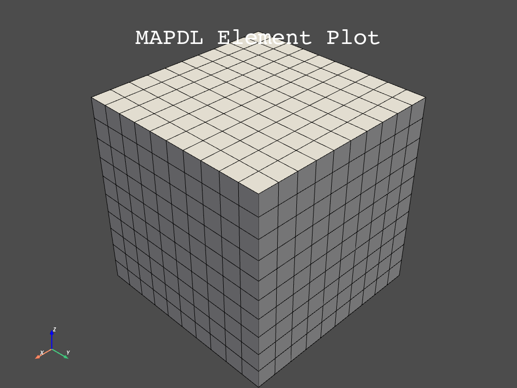
Meshing is quite easy, once the element and material are defined.
mapdl.esize(1 / 10)  # Element size
mapdl.vmesh(v0)
GENERATE NODES AND ELEMENTS
       IN VOLUMES       1  TO      1  IN STEPS OF      1

 NUMBER OF VOLUMES MESHED   =         1
 MAXIMUM NODE NUMBER        =      4961
 MAXIMUM ELEMENT NUMBER     =      1000
Let’s see the result
mapdl.eplot() # plot elements
Boundary conditions#
There are many boundary conditions options, and most of
them are applied using mapdl.d (for displacement)
or mapdl.f (for force).
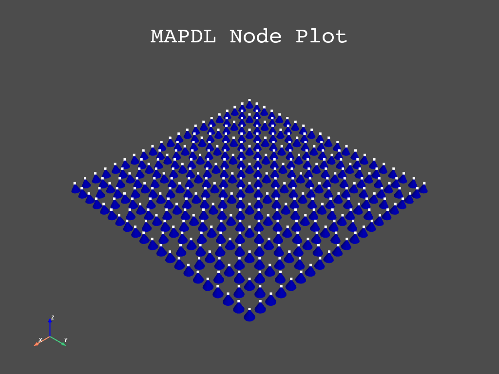
Let’s setup this example to represent a compression test. For that purpose, we need to fix the box bottom surface to have zero displacement.
But first, we need to select the corresponding nodes using
the mapdl.nsel command:
help(mapdl.nsel)
Help on method nsel in module ansys.mapdl.core._commands.database.selecting:

nsel(type_='', item='', comp='', vmin='', vmax='', vinc='', kabs='', **kwargs) method of ansys.mapdl.core.mapdl_grpc.MapdlGrpc instance
    Selects a subset of nodes.

    APDL Command: NSEL

    Parameters
    ----------
    type\_
        Label identifying the type of select:

        S - Select a new set (default).

        R - Reselect a set from the current set.

        A - Additionally select a set and extend the current set.

        U - Unselect a set from the current set.

        ALL - Restore the full set.

        NONE - Unselect the full set.

        INVE - Invert the current set (selected becomes unselected and vice versa).

        STAT - Display the current select status.


    The following fields are used only with Type = S, R, A, or U:

    Item
        Label identifying data. Valid item labels are shown in the table below. Some items also require a
        component label. If Item = PICK (or simply "P"), graphical picking is enabled and all remaining
        command fields are ignored (valid only in the GUI). Defaults to NODE.

    Comp
        Component of the item (if required). Valid component labels are shown in the table below.

    VMIN
        Minimum value of item range. Ranges are node numbers, set numbers, coordinate values, load
        values, or result values as appropriate for the item. A component name (as specified on the CM (p. 338)
        command) may also be substituted for VMIN (VMAX and VINC are ignored).

    VMAX
        Maximum value of item range. VMAX defaults to VMIN for input values. For result values, VMAX
        defaults to infinity if VMIN is positive, or to zero if VMIN is negative.

    VINC
        Value increment within range. Used only with integer ranges (such as for node and set numbers).
        Defaults to 1. VINC cannot be negative.

    KABS
        Absolute value key:

        - `kabs = 0` - Check sign of value during selection.
        - `kabs = 1` - Use absolute value during selection (sign ignored)

    Notes
    -----
    Selects a subset of nodes.  For example, to select a new set of nodes
    based on node numbers 1 through 7, do

    >>> mapdl.nsel('S','NODE','',1,7)

    The subset is used when the `'ALL'` label is entered (or implied)
    on other commands, such as

    >>> mapdl.nlist('ALL')

    Only data identified by node number are selected.  Data
    are flagged as selected and unselected; no data are actually deleted
    from the database.

    When selecting nodes by results, the full graphics value is used,
    regardless of whether PowerGraphics is on.

    Solution result data consists of two types, 1) nodal degree of freedom
    --results initially calculated at the nodes (such as displacement,
    temperature, pressure, etc.), and 2) element--results initially
    calculated elsewhere (such as at an element integration point or
    thickness location) and then recalculated at the nodes (such as
    stresses, strains, etc.).  Various element results also depend upon the
    recalculation method and the selected results location [AVPRIN, RSYS,
    FORCE, LAYER and SHELL].

    You must have all the nodes (corner and midside nodes) on the external
    face of the element selected to use Item = EXT.

    This command is valid in any processor.

    For Selects based on non-integer numbers (coordinates, results, etc.),
    items that are within the range VMIN-Toler and VMAX+Toler are selected.
    The default tolerance Toler is based on the relative values of VMIN and
    VMAX as follows:

    If VMIN = VMAX, Toler = 0.005 x VMIN.

    If VMIN = VMAX = 0.0, Toler = 1.0E-6.

     If VMAX ≠ VMIN, Toler = 1.0E-8 x (VMAX-VMIN).

    Use the SELTOL command to override this default and specify Toler
    explicitly.

    Table: 208:: : NSEL - Valid Item and Component Labels

    Table: 209:: : NSEL - Valid Item and Component Labels for Nodal DOF
    Result Values

    Examples
    --------
    Select nodes at `x == 0`, Of these, reselect nodes between ``1 < Y
    < 10``, then finally unselect nodes between ``5 < Y < 6``.

    >>> mapdl.nsel('S', 'LOC', 'X', 0)
    >>> mapdl.nsel('R', 'LOC', 'Y', 1, 10)
    >>> mapdl.nsel('U', 'LOC', 'Y', 5, 6)

    For other coordinate systems activate the coord system first.
    First, change to cylindrical coordinate system, select nodes at
    ``radius == 5``.  Reselect nodes from 0 to 90 degrees.

    >>> mapdl.csys(1)
    >>> mapdl.nsel('S', 'LOC', 'X', 5)
    >>> mapdl.nsel('R', 'LOC', 'Y', 0, 90)

    Note that the labels X, Y, and Z are always used, regardless of which
    coordinate system is activated. They take on different meanings in
    different systems Additionally, angles are always in degrees and
    NOT radians.

    Select elements assigned to material property 2

    >>> mapdl.esel('S', 'MAT', '', 2)

    Select the nodes these elements use

    >>> mapdl.nsle()

    Reselect nodes on the element external surfaces

    >>> mapdl.nsel('R', 'EXT')

    Change to cylindrical coordinates

    >>> mapdl.csys(1)

    Reselect nodes with radius=5

    >>> mapdl.nsel('R', 'LOC', 'X', 5)
mapdl.nsel("S", "loc", "z", 0)
mapdl.nplot()  # check the selection
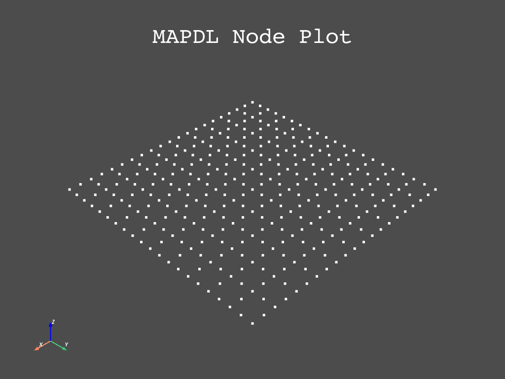
Applying to all selected nodes, displacement in Z direction equals to zero.
mapdl.d("all", "UZ", 0)

# Let's check the result
mapdl.nplot(plot_bc=True)
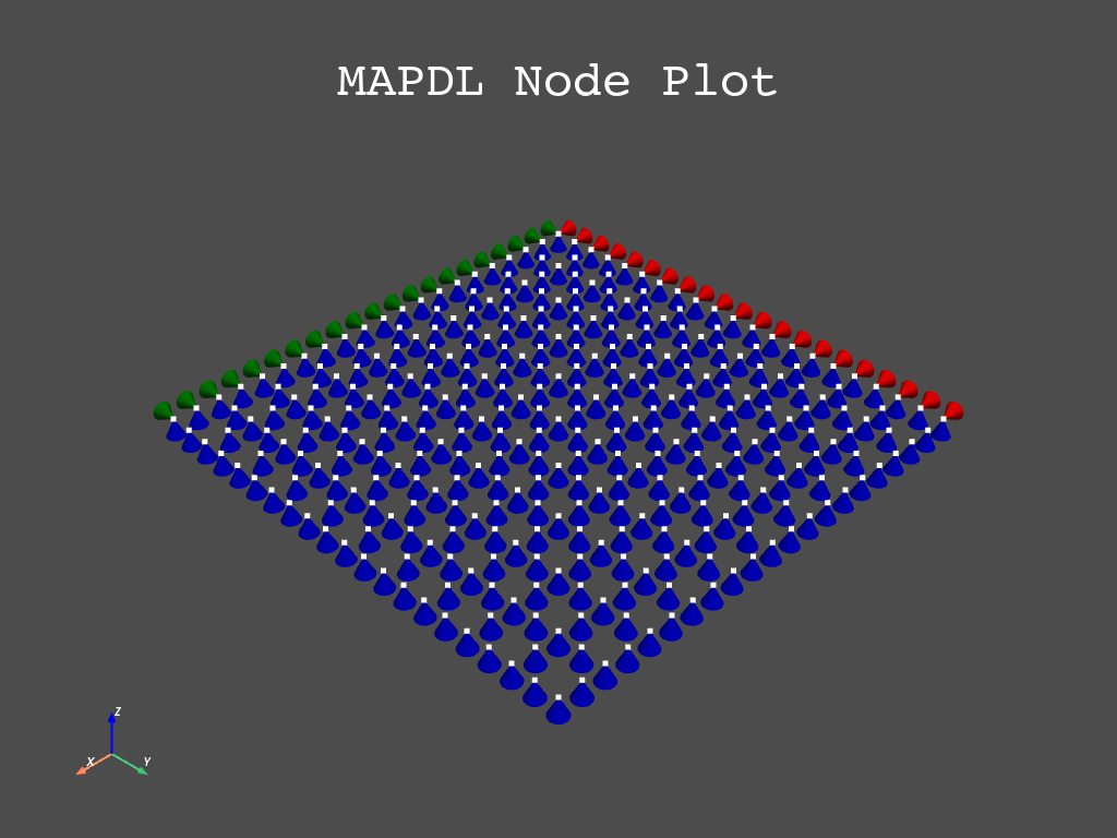
Let’s apply the rest of the boundary conditions.
# Let's fix the box edge XZ to not move except along Y.
mapdl.nsel("s", "loc", "z", 0)
# "r" is to reselect the nodes, from the previous "S" selection
mapdl.nsel("r", "loc", "x", 0)

mapdl.d("all", "UZ", 0)
mapdl.d("all", "UX", 0)

# we will do the same with the line YZ, but not move along X direction.
mapdl.nsel("s", "loc", "z", 0)
mapdl.nsel("r", "loc", "Y", 0)

mapdl.d("all", "UZ", 0)
mapdl.d("all", "UY", 0)
SPECIFIED CONSTRAINT UY   FOR SELECTED NODES            1 TO        4961 BY           1
 REAL=  0.00000000       IMAG=  0.00000000
Finally let’s fix one node in the directions:
mapdl.nsel("s", "loc", "x", 0)
mapdl.nsel("r", "loc", "y", 0)
mapdl.nsel("r", "loc", "z", 0)

mapdl.d("all", "all", 0)

# this code is redundant, because the nodal displacements do not overwrite each other
# if they are not in the same direction.
# This node was included in the previous lines selections, hence its
# boundary conditions are already defined.
SPECIFIED CONSTRAINT UX   FOR SELECTED NODES            1 TO        4961 BY           1
 REAL=  0.00000000       IMAG=  0.00000000
 ADDITIONAL DOFS=  UY    UZ
Let’s check the final result
mapdl.nsel("s", "loc", "z", 0)

mapdl.nplot(plot_bc=True)
Now let’s apply a displacement at the box top at each node. We could apply a force instead if we wish.
mapdl.nsel("s", "loc", "z", 1)
# mapdl.f("all", "FZ", 1E9)
mapdl.d("all", "UZ", 0.01)
SPECIFIED CONSTRAINT UZ   FOR SELECTED NODES            1 TO        4961 BY           1
 REAL= 1.000000000E-02   IMAG=  0.00000000
Analysis setup#
Let’s do a simple static analysis
mapdl.slashsolu()
mapdl.allsel()  # making sure all nodes and elements are selected.
mapdl.antype("STATIC")
output = mapdl.solve()
print(output)
*****  MAPDL SOLVE    COMMAND  *****

 *** NOTE ***                            CP =       1.569   TIME= 10:48:46
 There is no title defined for this analysis.

 *** SELECTION OF ELEMENT TECHNOLOGIES FOR APPLICABLE ELEMENTS ***
                ---GIVE SUGGESTIONS ONLY---

 ELEMENT TYPE         1 IS SOLID186. KEYOPT(2) IS ALREADY SET AS SUGGESTED.


 *** MAPDL - ENGINEERING ANALYSIS SYSTEM  RELEASE                  22.2     ***
 Ansys Mechanical Enterprise
 00000000  VERSION=LINUX x64     10:48:46  OCT 03, 2022 CP=      1.582


                       S O L U T I O N   O P T I O N S

   PROBLEM DIMENSIONALITY. . . . . . . . . . . . .3-D
   DEGREES OF FREEDOM. . . . . . UX   UY   UZ
   ANALYSIS TYPE . . . . . . . . . . . . . . . . .STATIC (STEADY-STATE)
   GLOBALLY ASSEMBLED MATRIX . . . . . . . . . . .SYMMETRIC

 *** NOTE ***                            CP =       1.586   TIME= 10:48:46
 Present time 0 is less than or equal to the previous time.  Time will
 default to 1.

 *** NOTE ***                            CP =       1.590   TIME= 10:48:46
 The conditions for direct assembly have been met.  No .emat or .erot
 files will be produced.

                      L O A D   S T E P   O P T I O N S

   LOAD STEP NUMBER. . . . . . . . . . . . . . . .     1
   TIME AT END OF THE LOAD STEP. . . . . . . . . .  1.0000
   NUMBER OF SUBSTEPS. . . . . . . . . . . . . . .     1
   STEP CHANGE BOUNDARY CONDITIONS . . . . . . . .    NO
   PRINT OUTPUT CONTROLS . . . . . . . . . . . . .NO PRINTOUT
   DATABASE OUTPUT CONTROLS. . . . . . . . . . . .ALL DATA WRITTEN
                                                  FOR THE LAST SUBSTEP


 SOLUTION MONITORING INFO IS WRITTEN TO FILE= file.mntr


                         ***********  PRECISE MASS SUMMARY  ***********

   TOTAL RIGID BODY MASS MATRIX ABOUT ORIGIN
               Translational mass               |   Coupled translational/rotational mass
         7800.0        0.0000        0.0000     |     0.0000        3900.0       -3900.0
         0.0000        7800.0        0.0000     |    -3900.0        0.0000        3900.0
         0.0000        0.0000        7800.0     |     3900.0       -3900.0        0.0000
     ------------------------------------------ | ------------------------------------------
                                                |         Rotational mass (inertia)
                                                |     5200.0       -1950.0       -1950.0
                                                |    -1950.0        5200.0       -1950.0
                                                |    -1950.0       -1950.0        5200.0

   TOTAL MASS =  7800.0
     The mass principal axes coincide with the global Cartesian axes

   CENTER OF MASS (X,Y,Z)=   0.50000       0.50000       0.50000

   TOTAL INERTIA ABOUT CENTER OF MASS
         1300.0      -0.41069E-11  -0.16058E-11
       -0.41069E-11    1300.0      -0.72902E-11
       -0.16058E-11  -0.72902E-11    1300.0
     The inertia principal axes coincide with the global Cartesian axes


  *** MASS SUMMARY BY ELEMENT TYPE ***

  TYPE      MASS
     1   7800.00

 Range of element maximum matrix coefficients in global coordinates
 Maximum = 1.914529915E+10 at element 247.
 Minimum = 1.914529915E+10 at element 556.

   *** ELEMENT MATRIX FORMULATION TIMES
     TYPE    NUMBER   ENAME      TOTAL CP  AVE CP

        1      1000  SOLID186      0.303   0.000303
 Time at end of element matrix formulation CP = 1.86823082.

 SPARSE MATRIX DIRECT SOLVER.
  Number of equations =       14159,    Maximum wavefront =    225
  Memory allocated for solver              =   113.349 MB
  Memory required for in-core solution     =   108.776 MB
  Memory required for out-of-core solution =    44.000 MB

 *** NOTE ***                            CP =       2.170   TIME= 10:48:46
 The Sparse Matrix Solver is currently running in the in-core memory
 mode.  This memory mode uses the most amount of memory in order to
 avoid using the hard drive as much as possible, which most often
 results in the fastest solution time.  This mode is recommended if
 enough physical memory is present to accommodate all of the solver
 data.
 Sparse solver maximum pivot= 7.658119658E+10 at node 4420 UY.
 Sparse solver minimum pivot= 4.423964031E+09 at node 672 UZ.
 Sparse solver minimum pivot in absolute value= 4.423964031E+09 at node
 672 UZ.

   *** ELEMENT RESULT CALCULATION TIMES
     TYPE    NUMBER   ENAME      TOTAL CP  AVE CP

        1      1000  SOLID186      0.225   0.000225

   *** NODAL LOAD CALCULATION TIMES
     TYPE    NUMBER   ENAME      TOTAL CP  AVE CP

        1      1000  SOLID186      0.045   0.000045
 *** LOAD STEP     1   SUBSTEP     1  COMPLETED.    CUM ITER =      1
 *** TIME =   1.00000         TIME INC =   1.00000      NEW TRIANG MATRIX


 *** MAPDL BINARY FILE STATISTICS
  BUFFER SIZE USED= 16384
       10.250 MB WRITTEN ON ASSEMBLED MATRIX FILE: file.full
        1.750 MB WRITTEN ON RESULTS FILE: file.rst
Post-Processing#
Let’s what we got. Let’s see the displacements:
mapdl.post_processing.nodal_displacement("all")
array([[ 0.     ,  0.     ,  0.     ],
       [-0.003  ,  0.     ,  0.     ],
       [-0.00015,  0.     ,  0.     ],
       ...,
       [-0.00285, -0.0027 ,  0.007  ],
       [-0.00285, -0.0027 ,  0.008  ],
       [-0.00285, -0.0027 ,  0.009  ]])
Let’s plot them
mapdl.post_processing.plot_nodal_displacement("Z")
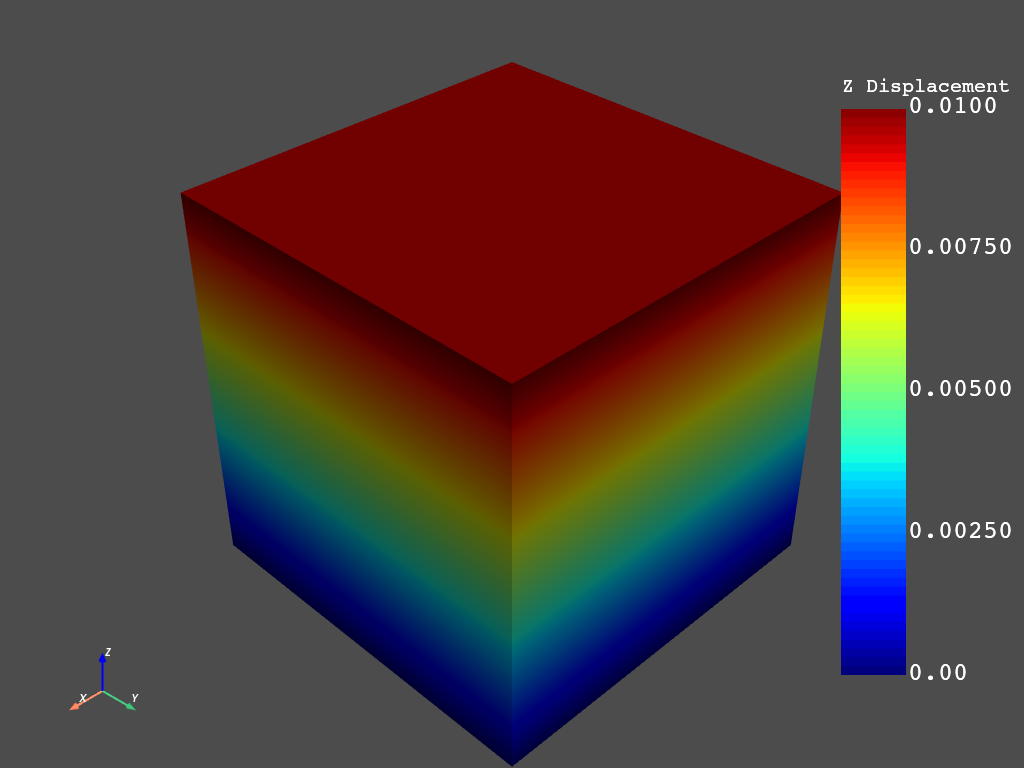
We can store the displacements as an array and use them for our calculations. For example:
nodal_disp = mapdl.post_processing.nodal_displacement("all")

print(f"The maximum displacement is {nodal_disp.max():0.3f}")
The maximum displacement is 0.010
Oh! By the way, you can format strings in this way, they are very powerful. This type of string is called f-string. The 0.3f after the colon (:) is the format for the number.
# First column is X displacement
print(f"The maximum X displacement is {nodal_disp[:, 0].max():0.3f}")

print(f"The average Z displacement is {nodal_disp[:, 2].mean():0.3f}")
The maximum X displacement is 0.000
The average Z displacement is 0.005
Closing session#
This is all for today. We hope you enjoyed this talk, as much as we enjoyed preparing it!
Closing PyMAPDL session
mapdl.exit()
Total running time of the script: ( 0 minutes 6.266 seconds)